APTOS 2019 Blindness Detection
Detect diabetic retinopathy to stop blindness before it’s too late
What is Diabetic Retinopathy (DR)?

Source: Medical Diagnosis with a Convolutional Neural Network, TowardsDataScience
According to this article:
- Diabetic retinopathy is the most common form of diabetic eye disease. Diabetic retinopathy usually only affects people who have had diabetes (diagnosed or undiagnosed) for a significant number of years.
- Retinopathy can affect all diabetics and becomes particularly dangerous, increasing the risk of blindness, if it is left untreated. -The risk of developing diabetic retinopathy is known to increase with age as well with less well controlled blood sugar and blood pressure level.
- According to the NHS, 1,280 new cases of blindness caused by diabetic retinopathy are reported each year in England alone, while a further 4,200 people in the country are thought to be at risk of retinopathy-related vision loss. All people with diabetes should have a dilated eye examination at least once every year to check for diabetic retinopathy.
Why Computer Vision (CV) for DR diagnosis?
According to the APTOS Kaggle Comptetion home page:
Millions of people suffer from diabetic retinopathy, the leading cause of blindness among working aged adults. Aravind Eye Hospital in India hopes to detect and prevent this disease among people living in rural areas where medical screening is difficult to conduct.
The need to AI:
Currently, Aravind technicians travel to these rural areas to capture images and then rely on highly trained doctors to review the images and provide diagnosis. Their goal is to scale their efforts through technology; to gain the ability to automatically screen images for disease and provide information on how severe the condition may be.
How doctors diagnose DR?
According to www.eyeops.com, doctors look for at least 5 patterns as in the image below:

Diabetic retinopathy can result in many serious issues affecting the blood vessels that nourish the retina., Source https://www.eyeops.com/
Diabetic retinopathy occurs when the damaged blood vessels leak blood and other fluids into your retina, causing swelling and blurry vision. The blood vessels can become blocked, scar tissue can develop, and retinal detachment can eventually occur.
AI that explains itself
In this work, I was particularly interested in using AI and CV (mainly ConvNets), and visualize the learnt patterns by the ConvNet feature maps, to see if similar patterns as above (Cotton wool spots, Hemorrhages, hard Exudates, Aneurysm and Abnormal growth of blood vessels), are also detected by ConvNets?
Data
The data is distributed as follows:
| Dataset | Number of scans |
|---|---|
| 3662 | 1928 |
Classes are: 0 - No DR
1 - Mild
2 - Moderate
3 - Severe
4 - Proliferative DR
Class imabalance
Before starting, very basic EDA shows class imabalnce issue:
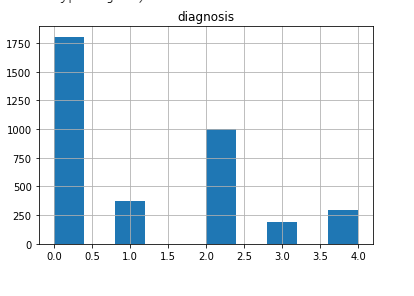
This is a common characteristic of many medical/healthcare datasets. The negative/normal case is usually the dominant one, which is intuitive. The positive cases are rare.
This issue will be treated later.
Evaluation metric
The metric used is Quadratic Weighted Kappa (QWKP). It is well explained in this kernel.
The wikipedia page offer a very concise explanation: “The weighted kappa allows disagreements to be weighted differently and is especially useful when codes are ordered. Three matrices are involved, the matrix of observed scores, the matrix of expected scores based on chance agreement, and the weight matrix. Weight matrix cells located on the diagonal (upper-left to bottom-right) represent agreement and thus contain zeros. Off-diagonal cells contain weights indicating the seriousness of that disagreement.”
The evaluation metric is of particular interest. The essence of QWKP is to favor prediction mistakes that are close to the correct answer than the ones far from it. In other words, if the correct class is “Mild”, while the prediction is “Moderate”, this is better than if the prediction is “Severe”. This is intuitive, specially for “Ordinal” target variables, where classes represent a mark on an ordered discrete scale, representing severity as in our case. This is a common case in many medical diagnosis problems, like in Radiology or Lab reports for example.
If you navigate in the Kaggle kernels of APTOS competetion, you will see three main approaches to specify the loss function and network output. This relates to problem formulation as one of the following:
| Problem | Loss | Network output | Comment | Example |
|---|---|---|---|---|
| Multi-class | Cross Entropy | Softmax/Class probabilities | Normal choice. But not good for QWKP, since CE favors only the correct class | Kaggle kernel |
| Regression | RMSE | Linear/Relu | If RMSE is small enough, this is good since the error/confusion will at max to the neighbor class | Kaggle kernel |
| Multi-label | Binary Cross Entropy | Sigmoid | By formatting the ground truth labels such that the label is all ones until the correct prediction then all 0’s. This encourages the model to output the correct class or at least the neighboring ones | Kaggle kernel |
In theory, formulating the problem as regression or multi-label classification seems better than multi-class classification, since cross entropy loss always focus on errors that caused the correct label not to be predicted, and hence optimizing in that direction. In other words, if the prediction is the class next to the correct one, this makes no difference to the cross entropy loss.
On contrary, the regression RMSE loss, would try to output the correct number +/- some error (RMSE). If this error is small enough, then at worst we get confused only to the neighbor class. This is good to QWKP score.
Also, multi-label formulation would format the targets as follows: 0 –> 1,0,0,0,0
1 –> 1,1,0,0,0
2 –> 1,1,1,0,0
3 –> 1,1,1,1,0
4 –> 1,1,1,1,1
Which can be visualized as an ascending progress bar, representing severity. The loss is then Binary Cross Entropyt (BCE) over each output neuron (Sigmoid). This should encourage the model to output high values at the correct class, or at worst around it, which is also good for QWKP.
The problem with this approach is the decoding process. In normal cases, we would take the index of the last predicted 1 in the output, which is immediately followed by 0. The assumption here is that the model never outputs a 0 followed by 1, which breaks the ordered progress bar. Imagine that the model outputs by mistake [0,1,1,1,0], our approach would estimate the fourth class Severe, which the correct one might be No DR, which is a bad diagnosis and hurts the QWKP. Fortunately this cases is rare for a well trained model.
Surprisingly, the three formulations are almost the same in practice, in terms of QWKP! Although the last two seem more intuitive. However, the above discussion aims at triggering to consider the 3 approaches when dealing with ordinal targets prediction.
In the work below, we use the multi-class formulation.
Model
ConvNet model
Some ideas in the code are insipred by this Kaggle kernel.
Small custom model
As a start, trying a simple small Conv2D model seems to perform fairly good:
from tensorflow.keras import layers
from tensorflow.keras import models

model = models.Sequential()
model.add(layers.Conv2D(32, (3, 3), activation='relu',
                        input_shape=(sz, sz, 3)))
model.add(layers.MaxPooling2D((2, 2)))
model.add(layers.Conv2D(64, (3, 3), activation='relu'))
model.add(layers.MaxPooling2D((2, 2)))
model.add(layers.Conv2D(128, (3, 3), activation='relu'))
model.add(layers.MaxPooling2D((2, 2)))
model.add(layers.Conv2D(128, (3, 3), activation='relu'))
model.add(layers.MaxPooling2D((2, 2)))

model.add(layers.Flatten())
model.add(layers.Dense(512, activation='relu'))
model.add(layers.Dense(n_classes, activation='softmax'))
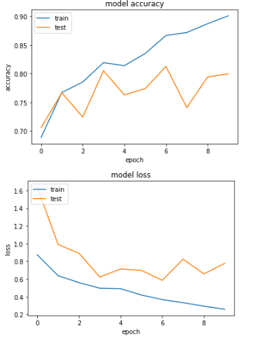
![imgs/small_model_curves.png]
Looking on the learning curve, the models seems to perform well. No sign of overfitting. It’s the opposite actually, test results are better. This encourages to have a bigger model capacity.
However, this result is tricky. The accuracy is good because of the majority classes dominating. This advises against depending on accuracy
QWKP is around 0.77. Looking on the leaderboard, the top QWKP was around 0.93. Which means the simple model is performing poorly.
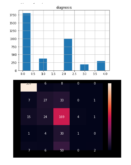
Visualization of learnt features
Let’s look on the learnt features anyway. We will use Grad-CAM method. For more implementation details, please see this colab.
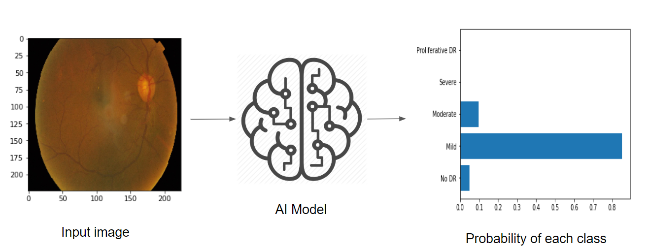
It is clear from the confusion matrix, how class (0=No DR) and (2=Moderate), dominate the predictions. This is also clear in the visualizations, where the main learnt features is the pupile location, which is the dominant feature of the negativ/normal classes that dominate the data.
In some cases, the confusion is slight (see the probabilities of 2 and 3 are close) In such cases, the features are very good (cotton patterns are detected).

In some cases, although correctly classified, but the features capture small nodules. Not sure if this is due to sensitivity to small variations, or it’s correct retina feature? Needs a specialist!

In other cases, the features actually reflects luminance/light or shadows effects. This is reflects high sensitivity of the learnt features, so it’s not capturing the class specific features.
ResNet50 model
As suggested by the learning curves, we move to a bigger pre-trained model. We use ResNet50 backend, GlobalAveragePooling, and add few classification layers.
inp = layers.Input(shape=(sz,sz,3))
conv_base = ResNet50(include_top=False,
               weights='imagenet',
               input_tensor=inp)

x = layers.GlobalAveragePooling2D()(conv_base.output)
x = layers.Dropout(0.5)(x)
x = layers.Dense(1024, activation='relu')(x)
x = layers.Dropout(0.5)(x)
out = layers.Dense(n_classes, activation='softmax')(x)
model = models.Model(inp, out)
The normal fine-tuning scenario would be:
- Freeze the conv_base (ResNet)
- Warm-up: train only the top layers
- Unfreeze the conv_base
- Fine tune top layers, or all conv_base
However, in our case, ImageNet is completely different from APTOS data. So we have to fine tune the whole conv_base.
Treating class imbalance
We use the cost-sensitive approach to treat class imabalance. In other words, we weight the minority class higher in the loss function, which has a similar effect to oversampling the minority samples. Data augmentation of the minority class only would cause bias in the model.
We use the class_weight argument of the fit function in tensorflow.keras. To find the class weights we use sklearn.utils.class_weights:
from sklearn.utils import class_weight
class_weights = class_weight.compute_class_weight('balanced', sorted(classes), y)
This is exactly equivalent to the following code:
s = sum(classes_cnts)
n = len(classes)
class_weights = np.array([s/(n*classes_cnts[cl]) for cl in sorted(classes)])
In both cases, we weight the class of higher count less, scaled by the total number of classes / total samples.
Optimization/Callbacks
ReduceLROnPlateau
Using the tensorflow.keras.callbacks.ReduceLROnPlateau improves the results a lot, where the optimizer reduces the learning rate by a the argument factor, whenever the loss is not improving for some epochs decided by the patience argument. This prevents the model from overfitting. Short patience=2 gives better results, since it tends to smooth the learning curve and prevent overfitting early.
Cyclic Learning Rate
We used also the cyclic learning rate adjustment (see Leslie Smith paper), with Traingular2 pattern:
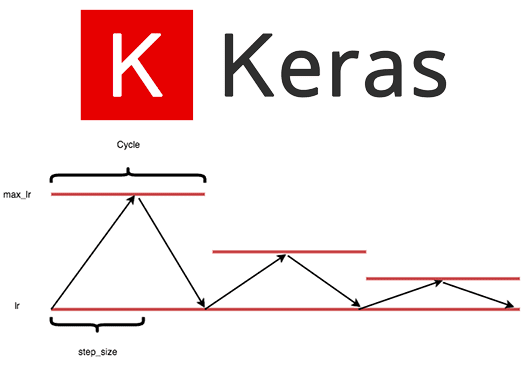 .
.
In Keras, we use tensorflow_addons.optimizers.CyclicalLearningRate callback :
cyc_lr_schedule = tfa.optimizers.CyclicalLearningRate(#optimizers.schedules.CyclicalLearningRate(
    initial_learning_rate=1e-4,
    maximal_learning_rate=1e-2,
    step_size=2000,
    scale_fn=lambda x: 1.,
    scale_mode="cycle",
    name="MyCyclicScheduler")
Which can later be used with any optimizer:
optimizers.Adam(learning_rate=cyc_lr_schedule)
The result of QWKP is almost the same of ReduceLROnPlateau callback, but at slower and more smooth learning pattern.
Learning Rate Finder
To decide on the initial learning rate, we used LRFinder callback, following also Leslie Smith paper. For more details see this colab.
This gives the same initial learning rate we used (=1e-4), for both RMSprop and Adam.
Learning curves
Doing the above improvements we get the following learning curves:
The test accuracy improves to 81%, while the QWKP reaches around 0.88, which is close enough to the leaderboard (0.93).
The model overfits around epoch 6. Without the ReduceLROnPlateau, overfitting happpens around epoch 2-3, with QWKP=0.79. With more regularization, we could get closer to the leaderboard.
Confusion matrix
After treating the class imbalance, let’s have a look on the confusion matrix:
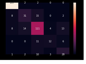
As can be seen, the confusion is much less severe. The diagonal in all classes is the dominant number. However, confusions are still going to far dominant classes, like (4=Severe) mostly confused to (2=Moderate), which still hurts the QWKP. Further light oversampling/augmentation of class 4 could help (to be tried later).
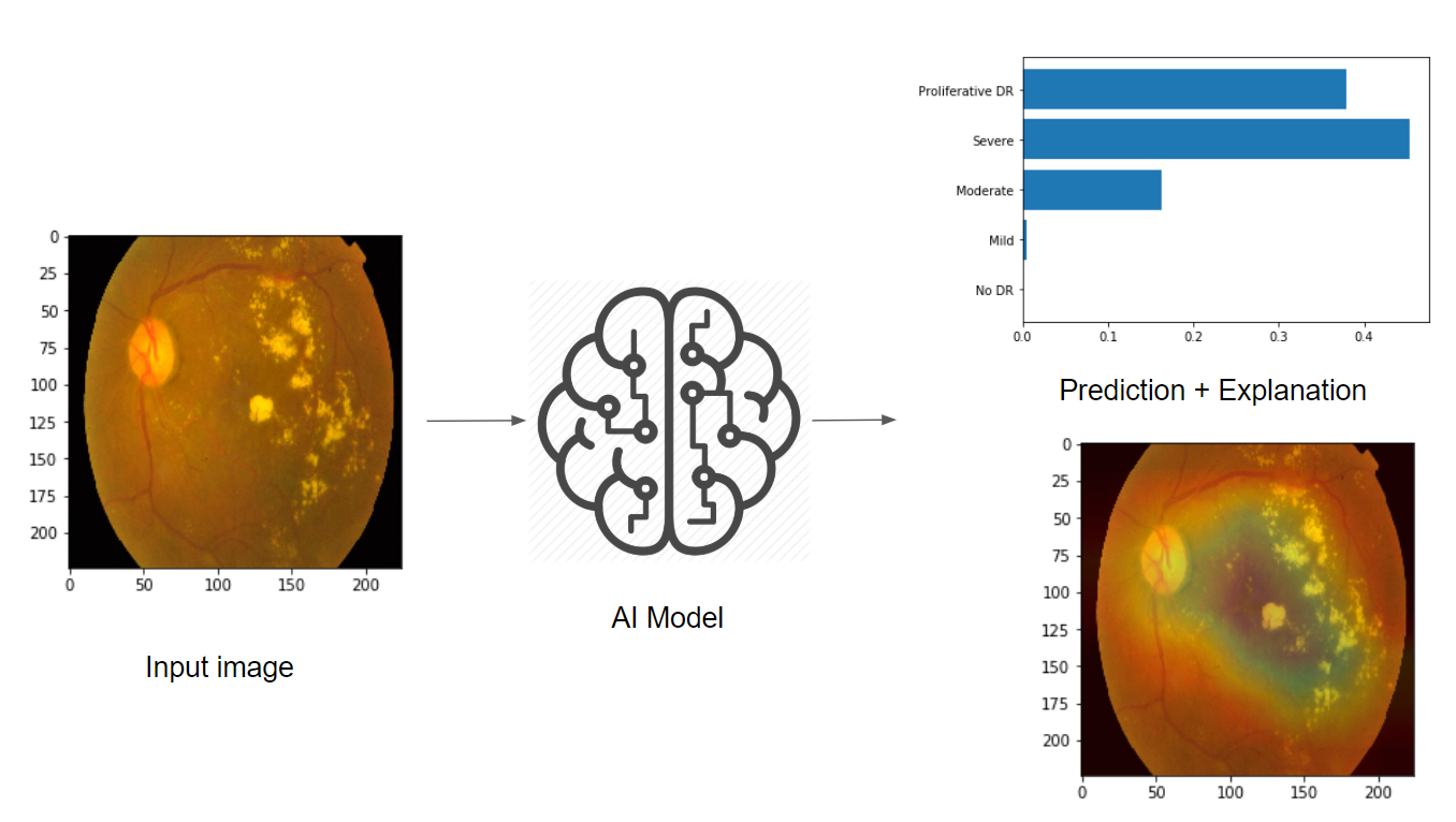
Visualization of learnt features
Let’s have a look on the learnt features.
In ResNet, the final feature maps are course grids of 7x7. Spreading these on the input image 224x224 might have coarse features (like ink spelt on paper).
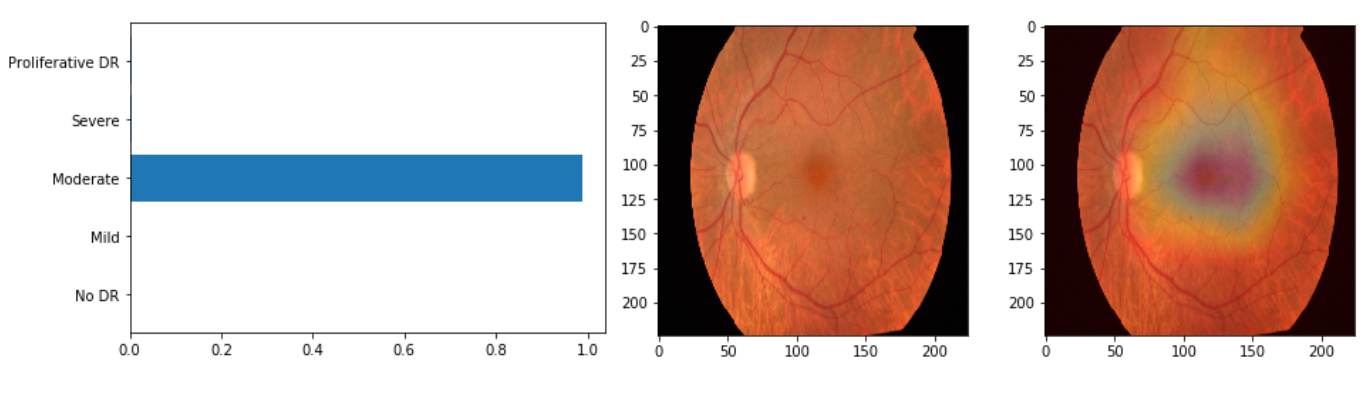
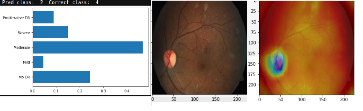
In the above case, the correct class is (1=Mild) but the prediction is (2=Moderate). This won’t hurt the QWKP a lot, moreover, it’s justified looking on the spot leading to this prediction. So the model becomes to make more sense.
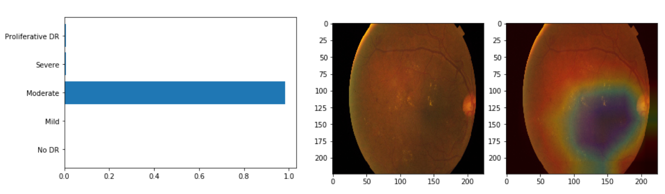
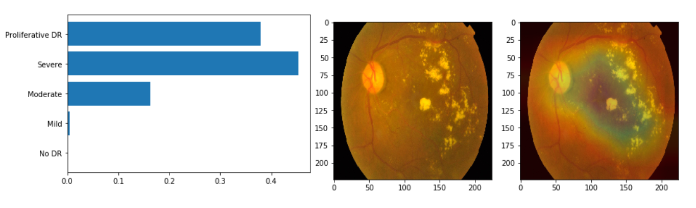
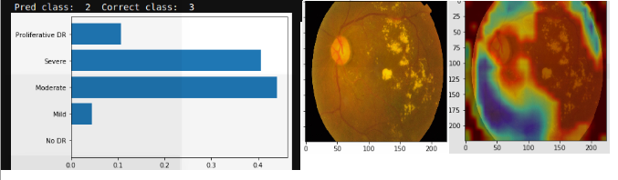
The above two predictions are correct. The defective patterns are stil detected, without particular attention to the pupil feature (which is common in all classes so it’s not good to detect). This is a good sign.
Moreover, probabilities become more within a local region of classes, which justifies the good QWKP result.
Conclusion
In this tutorial, we went through an important application of computer vision, which is medical imaging diagnosis, in this case the Diabetic Retina. The visualization of the learnt feature maps using Grad-CAM method explains a lot of features, according to the well known DR patterns. The metric used in this competetion is interesting, and gives an idea about the importance of choosing the good metric for such kind of problems of predicting ordinal target variables. Also, this application exposes us to some important problems in ML like class imbalance, which is common in healthcare and medical diagnosis problems. Some tricks like class weighted loss, reducing learning rate on plateau, cyclic learning rate,…etc improve the QWKP with around 10%.
Important note:
I’m not a doctor to judge, so the visualizations here might be completely random features in the end. However, the good QWKP results suggest that the model captured good results. But it should be emphasized that, a more trained expert eye should validate those assumptions.