LiDAR Sensor Modeling and Data Augmentation with CycleGAN

Artificial Intelligence is disrupting the automotive industry these days. With the rush to deploy autonomous cars, car manufacturers and suppliers are racing to integrate deep learning algorithms in their products, ranging from end-to-end applications to environment perception (object detection, semantic segmentation,…etc) which is the nearest to deployment. However, deep learning models are monsters known for their data hunger, and their favorite is “real” data, which means in more technical terms: training data that come from the same distribution as the deployment or test data. But we cannot always feed them their favorite dish for some reasons:

• Real data collection is expensive and sometimes unsafe.
• Real data annotation is also expensive and complicated for many sensors.

LiDAR

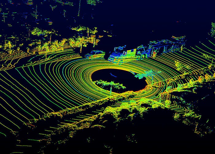
The autonomous vehicle is equipped with all types of sensors, Camera, LiDAR, Radar, Ultrasonic…etc. While Camera is the most famous sensor, with rich legacy of research ideas and data sets, other sensors, like LiDAR (Light Detection And Ranging) do not enjoy the same luxury. LiDAR sensors are far more expensive than Camera. Moreover, LiDAR data is often processed in their raw 3D Point Cloud (PCL) form resulting from the laser beam scanning the surroundings, and providing a list of points in the 3D space, each indicating the location of the reflection on surrounding objects.

Such special nature induces two other downsides: 1) data annotation becomes complex, as it requires better understanding by the human annotator of the nature of the signal at hand and 2) the maturity of perception algorithms based on LiDAR is far beyond their Camera peers which are often developed for the familiar 2D perspective Camera views.

Sensor models

One trick to overcome such limitations is to use synthetic data from simulators and game engines as training data, or at least to augment the “few” real data. Such data enjoy “free” annotations coming from the simulator engine, and can be generated for difficult scenarios that do not frequently occur in reality, like different traffic, weather, day/night conditions or even in accidents and corner cases simulations. But the main problem with simulators is that they are “too perfect”! For example, realistic LiDAR suffers from noise due to dust, rain, humidity,…etc, and sometimes reflections are not perfect or the beam diverges a little with distance. All those imperfections make the real LiDAR PCL look different from the perfect simulated one. To make the generated LiDAR look realistic, we need to develop what is called a “sensor model”, which imitate all those conditions, and try to produce realistic LiDAR PCL for the simulated one. In this way, the sensor model perceives the simulated environment “as if” a real LiDAR sensor did it.

But the question is: how to define the parameters of such a model?

One can think of developing closed form models for all those variables of imperfections, but the reality is: it’s very hard to formulate! The other way is to learn such sensor model. Learning the sensor model cannot be done through the traditional supervised learning framework, because we do not have a data set of x (the clean LiDAR) and its corresponding y (the noisy LiDAR), which is called a “paired” data set. If we have such a dataset, then our problem is solved! However, we can have “unpaired” data of simulated LiDAR, and another one for real LiDAR.

The question now is: how to learn a mapping between the two domains given the unpaired data?

The answer is unpaired image-to-image translation. Generative Adversarial Networks (GANs) (Goodfellow et al., 2014) have recently shown great performance in this domain, with CycleGAN (Zhu et al., 2017a), UNIT (Liu et al., 2017).

CycleGAN for LiDAR domains translations

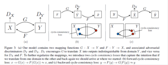
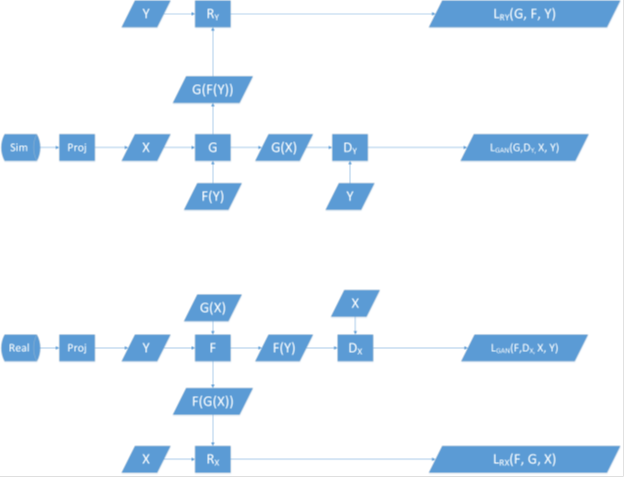
In our recent paper, we employ CycleGANs. In CycleGAN, we have two domains to translate between (two-way), domain A and domain B. The model learns two generators (G and F) and two discriminators (D_X and D_Y). The function of the generators is to make the translation in either way, and fool the discriminators, which try to distinguish if their input is coming from their domain or the other one. In addition, an extra loss is added, to see if each translated domain can be reconstructed back to its origin or not, called the Cycle Consistency Loss.

We formulate the problem of LiDAR sensor modeling as domain translations, with domain A being the LiDAR PCL produced from CARLA simulator, while domain B is the realistic LiDAR PCL coming from KITTI dataset.

LiDAR projections

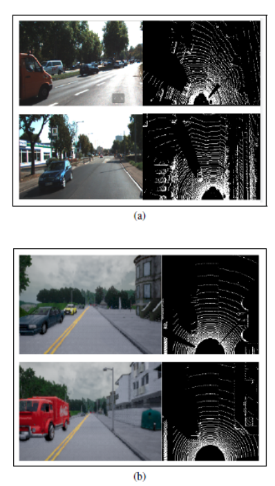
How to feed the 3D LiDAR PCL to the CycleGAN model which accepts 2D inputs?We use two projection methods of the 3D PCL on 2D views, each encodes a 2D “occupancy map”, where each “pixel” location indicates a location in space, while its value indicates different this according to the mapping technique:

• Bird-Eye-View (BEV): where the LiDAR PCL is projected in the top view, and the space around the vehicle is fragmented into a matrix of 2D cells or bins, each indicating a location. The resolution of the map indicates the cell size. Each 3D LiDAR point is projected in one of those cells. Such a 2D map will now include either “0” if no point falls into it, or “1” if there is at least one point falls into it. Another encoding could be to keep the highest point value in the vertical direction as the cell value.

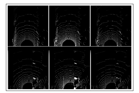
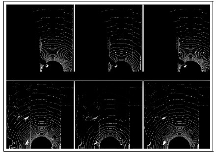
• Polar-Grid-Map (PGM): The way the LiDAR scans the environment is by sending multiple laser rays in the vertical direction, which define the number of LiDAR channels or layers. Each beam scans a plan, in the horizontal radial direction with a specific angular resolution. A LiDAR sensor configuration can be defined in terms of the number of channels, the angular resolution of the rays, in addition to its Field of View (FoV). PGM takes the 3D LiDAR point cloud and fit it into a 2D grid of values. The rows of the 2D grid represent the number of channels of the sensor (For example, 64 or 32 in case of Velodyne). The columns of the 2D grid represent the LiDAR ray step in the radial direction, where the number of steps equals the FoV divided by the angular resolution. The value of each cell is ranging from 0 to 1 describing the distance of the point from the sensor. Such an encoding has some advantages. First, all the 3D LiDAR points are included in the map. Second, there is no memory overhead, like Voxelization for instance. Third, the resulting representation is dense, not sparse.

LiDAR translations

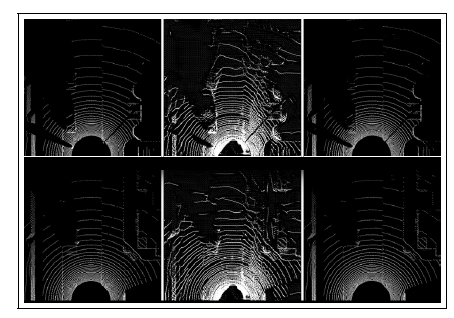
• Sim2Real: we can perform LiDAR translation from the CARLA simulator frames to the realistic KITTI frames (CARLA2KITTI) and vice versa (KITTI2CARLA). This can be done both in BEV and PGM projections.

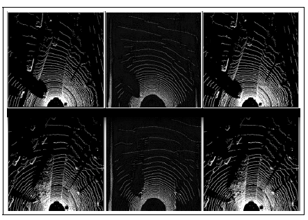
• Real2Real: we can also perform the translation between different sensors models configurations. In particular, we test the ability of CycleGAN to translate from a domain with few LiDAR channels (32) to another domain with denser channels (64). The main advantage of this translation is that, dense sensors like Velodyne are expensive and bulky. With this translation with CycleGAN, we can have small LiDAR sensors, with few layers, and we can synthesize the dense LiDAR from it.

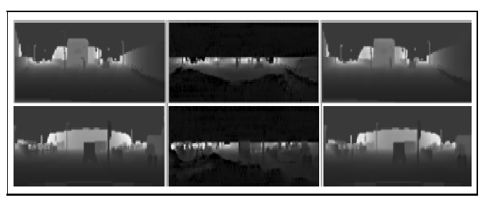
• Sensor2Sensor: we can also map directly from Camera frames into LiDAR domain (CAM2LIDAR). The gain here is huge; imagine a car that is not equipped with LiDAR, but only Camera, we can collect Camera data, and use any well-known network to annotate, say objects, then use CycleGAN to translate that into LiDAR. In that way, we have LiDAR data without even having any expensive LiDAR installed in the car!

How to evaluate the quality of the generated PCL?

Thus far, the only way to evaluate the quality of the generated LiDAR is either subjective, through human judgment, or intrinsic, through the quality of the reconstruction in sim2real setup (CARLA2KITTI), or real2sim setup (KITTI2CARLA).

As a step towards a quantitative extrinsic assessment, one can think of using an external “judge,” that evaluates the quality of the generated LiDAR in terms of the performance on a specific computer vision task, object detection for instance. The evaluation can be conducted using a standard benchmark data set YObj , which is manually annotated like KITTI. For that purpose, an object detection network from LiDAR is trained, following YOLO3D (Ali et al., 2018) and YOLO4D (El Sallab et al., 2018). Starting from simulated data X, we can get the corresponding generated Y data using G. We have the corresponding simulated data annotations YObj . Object detection network can be used to obtain Y^Obj , which can be compared in terms of mIoU to the exact YObj . Moreover, Object detection network can be initially trained on the real benchmark data, KITTI, and then augment the data with the simulator generated data, and the mIoU can be monitored continuously to measure the improvement achieved by the data augmentation.

How to ensure the important environment objects still exist in the translated map?

In essence, we want to ensure that, the essential scene objects are mapped correctly when transferring the style of the realistic LiDAR. This can be thought as similar to the content loss in the style transfer networks. To ensure this consistency, an extrinsic evaluation model is used. We call this model a reference model. The function of this model is to map the input LiDAR to a space that reflects the objects in the scene, like semantic segmentation or object detection networks. For instance, this network could be YOLO network trained to detect objects from LiDAR views. In more technical terms, we want to augment the cycle consistency losses with another loss that evaluates the object information existence in the mapped LiDAR from simulation to realistic.

Conclusion

We tackled the problem of LiDAR sensor modeling in simulated environments, to augment real data with synthetic data. The problem is formulated as an image-to-image translation, where CycleGAN is used to map sim2real and real2real. KITTI is used as the source of real LiDAR PCL, and CARLA as the simulation environment. The experimental results showed that the networks able to translate both BEV and PGM representations of LiDAR. Moreover, the intrinsic metrics, like reconstruction loss, and visual assessments show a high potential of the proposed solution. We discuss in the future works a method to evaluate the quality of the generated LiDAR, and also we presented an algorithm to extend the Vanilla CycleGAN with a task-specific loss, to ensure the correct mapping of the critical content while doing the translation.